Simulating two crossing bundles

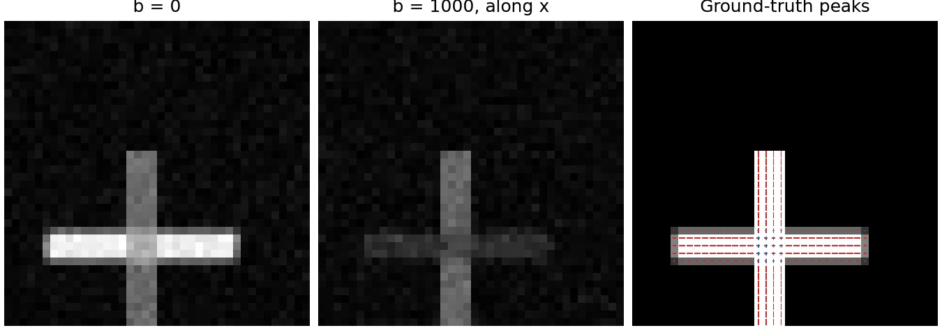
This example builds two straight fibre bundles that cross at 90 degrees, simulates their diffusion-weighted images with noise, saves the result with save_simulation, and draws the b = 0 image, one diffusion-weighted image and the ground-truth fibre directions.

A phantom is an object to scan. It is made of tissues, each with compartments that have their own diffusion and relaxation, and fibre bundles that place the tissues on a voxel grid. simulate turns a phantom into diffusion-weighted images with the instant engine, which evaluates the signal of each voxel in closed form. It also keeps the ground truth: how much of each voxel each tissue and bundle fills, and where the fibres point.

The two bundles here have different parameters of the standard model of white matter and different T2, so the b = 0 image tells them apart. The scan has one b = 0 volume and one shell of 32 directions at b = 1000 s/mm^2.

The simulation builds on SymDWI, by the same author. The models and their papers are listed in the Background page on simulation.

import tempfile
from pathlib import Path

import numpy as np
from matplotlib.figure import Figure

from larmor.io import load_volume
from larmor.simulation import (
    Bundle,
    BundleGeometry,
    Phantom,
    Protocol,
    create_gradient_table,
    save_simulation,
    simulate,
    standard_model_tissue,
)
from larmor.types import Grid

The bundles

The phantom is a 40 x 40 x 40 grid of 1 mm voxels. The first bundle runs along x. The second is 25 mm long, crosses the first at its middle and runs along y, so the crossing is at 90 degrees. Control points and radii are in mm, in world coordinates. The seeds make the streamlines the same on every run.

grid = Grid((40, 40, 40), np.eye(4))

first = BundleGeometry(
    np.array([[5.0, 10.0, 10.0], [17.5, 10.0, 10.0], [30.0, 10.0, 10.0]]),
    num_streamlines=1000,
    radius=2.0,
    seed=1,
)
half = 12.5 * np.array([0.0, 1.0, 0.0])
middle = np.array([17.5, 10.0, 10.0])
second = BundleGeometry(
    np.array([middle - half, middle, middle + half]),
    num_streamlines=1000,
    radius=2.0,
    seed=2,
)

The tissues

Each bundle is filled by a white matter tissue made of a stick (intra-axonal water) and a zeppelin (extra-axonal water). The second has a lower axial and a higher radial diffusivity, and shorter T2 times, so it is darker at b = 0.

wm1 = standard_model_tissue(
    name="WM1",
    intra_fraction=0.75,
    intra_diffusivity=1.7e-3,
    extra_parallel_diffusivity=1.7e-3,
    extra_perpendicular_diffusivity=0.35e-3,
    intra_t2_ms=90.0,
    extra_t2_ms=60.0,
)
wm2 = standard_model_tissue(
    name="WM2",
    intra_fraction=0.75,
    intra_diffusivity=1.5e-3,
    extra_parallel_diffusivity=1.3e-3,
    extra_perpendicular_diffusivity=0.75e-3,
    intra_t2_ms=50.0,
    extra_t2_ms=30.0,
    t2star_ms=35.0,
)
phantom = Phantom(
    grid,
    tissues=(wm1, wm2),
    bundles=(Bundle(first, tissue="WM1"), Bundle(second, tissue="WM2")),
)

The scan

The scan has one b = 0 volume and 32 directions at b = 1000 s/mm^2. The pulses are 15 ms long and 30 ms apart, the echo time is 80 ms and the repetition time 3000 ms.

gradients = create_gradient_table([(1000, 32)], num_b0=1, seed=0)
protocol = Protocol(gradients, 15.0, 30.0, 80.0, 3000.0)

Simulating

With an SNR of 30 the noise level is a thirtieth of the b = 0 signal of a voxel filled with WM1, and it is the same in every voxel. The same seed gives the same images.

result = simulate(phantom, protocol, snr=30, noise_reference="WM1", seed=0)
dwi = result.echoes[0].data
print(f"DWI: {dwi.shape}, noise sigma {result.sigma:.4f}")

for name, voxel in (("first bundle only", (8, 10, 10)), ("crossing", (17, 10, 10))):
    print(f"b = 0 signal, {name}: {result.noise_free[0].data[voxel][0]:.3f}")

DWI: (40, 40, 40, 33), noise sigma 0.0085
b = 0 signal, first bundle only: 0.255
b = 0 signal, crossing: 0.185

The files

save_simulation writes one folder. It holds the images with their bvals and bvecs, the ground truth, the bundles, and the phantom file with the protocol, which lar simulate can run again. The ground-truth peaks are in the layout that lar peaks writes: 3 volumes per peak, each peak’s direction scaled by its amplitude.

with tempfile.TemporaryDirectory() as folder:
    files = save_simulation(result, folder)
    print(sorted(path.name for path in Path(folder).iterdir()))
    peaks = load_volume(files.peaks).data

crossing = peaks[17, 10, 10].reshape(-1, 3)
cosine = abs(crossing[0] @ crossing[1]) / np.prod(np.linalg.norm(crossing[:2], axis=1))
print(f"Peaks at the crossing: {np.degrees(np.arccos(cosine)):.0f} degrees apart")

['background_fraction.nii.gz', 'bundle_1.tck', 'bundle_2.tck', 'bundle_fractions.nii.gz', 'compartment_fractions.nii.gz', 'dwi.bval', 'dwi.bvec', 'dwi.nii.gz', 'dwi_noise_free.nii.gz', 'free_water_fraction.nii.gz', 'free_water_signal_fraction.nii.gz', 'mask_WM1.nii.gz', 'mask_WM2.nii.gz', 'mask_bundles.nii.gz', 'peaks.nii.gz', 'phantom.json', 'signal_fractions.nii.gz', 'simulation.json', 'tissue_fractions.nii.gz']
Peaks at the crossing: 90 degrees apart

The images and the ground truth

The plane z = 10 holds both bundles. At b = 0 the first, with the longer T2, is brighter. With the gradient along x, the first bundle loses most of its signal, since its fibres run along the gradient, and the second, across it, loses less. Both images share one grey scale. The third panel draws the ground-truth peaks as lines, red for the largest peak of a voxel and blue for the next, over the fraction of the voxel the bundles fill. The figure is drawn with matplotlib.

along_x = int(np.argmax(np.abs(gradients.bvecs[1:, 0]))) + 1
planes = [
    dwi[:, :, 10, 0],
    dwi[:, :, 10, along_x],
    result.partition.tissue_fractions[:, :, 10].sum(axis=-1),
]
titles = ["b = 0", "b = 1000, along x", "Ground-truth peaks"]
figure = Figure(figsize=(9, 3.2), layout="constrained")
for axes, plane, title in zip(figure.subplots(1, 3), planes, titles, strict=True):
    top = planes[0].max() if plane is not planes[2] else 1.0
    axes.imshow(plane.T, origin="lower", cmap="gray", vmin=0, vmax=top)
    axes.set_title(title)
    axes.set_axis_off()
x, y = np.meshgrid(np.arange(40), np.arange(40), indexing="ij")
for k in range(0, peaks.shape[3], 3):
    u, w = peaks[:, :, 10, k], peaks[:, :, 10, k + 1]
    figure.axes[2].quiver(
        x,
        y,
        u,
        w,
        angles="xy",
        scale_units="xy",
        scale=1.2,
        pivot="mid",
        headwidth=0,
        headlength=0,
        headaxislength=0,
        color="tab:red" if k == 0 else "tab:blue",
        width=0.004,
    )
figure.savefig("simulate_crossing_bundles.png", dpi=150)