The signal of one voxel, step by step

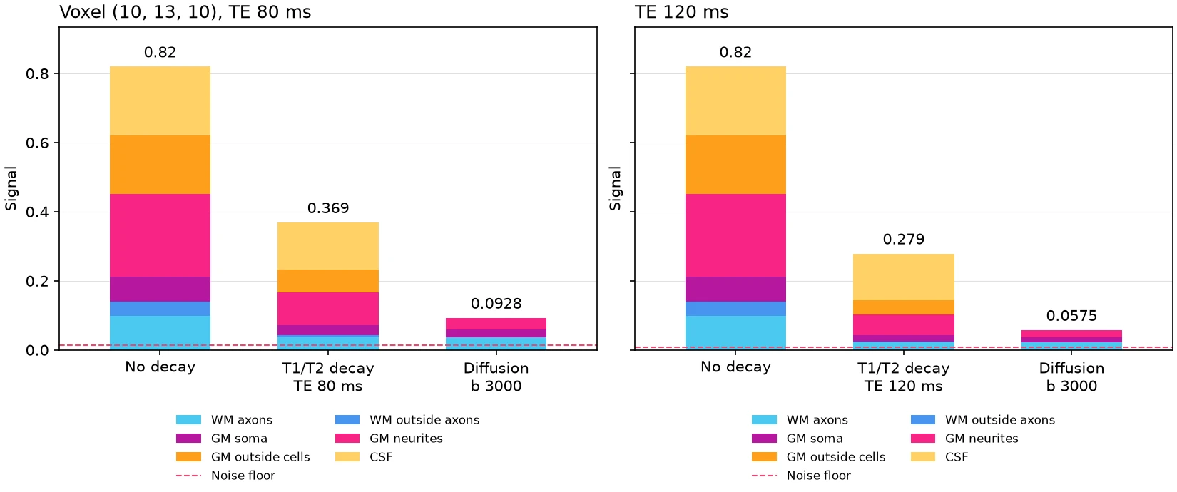
This example builds a white matter bundle that fills part of a voxel of grey matter, draws how that voxel’s signal at b = 3000 s/mm^2 is built from its factors, and then shows how a longer echo time changes it.

A simulated image shows only the product of many factors: how much of the voxel each tissue fills, the tissue’s proton density, the T1 and T2 relaxation, and the diffusion attenuation of each compartment. signal_breakdown splits the signal of one voxel in one volume into these factors, with the same compartment models as simulate, and plot_signal_breakdown draws it as three stacked bars: the water with no decay, the signal after the T1 and T2 decay, and the signal after the diffusion weighting.

import numpy as np
from matplotlib.figure import Figure

from larmor.plot import plot_signal_breakdown
from larmor.simulation import (
    Bundle,
    BundleGeometry,
    Phantom,
    Protocol,
    TissueMap,
    create_gradient_table,
    partition_voxels,
    signal_breakdown,
)
from larmor.types import Grid, Volume

The phantom

The phantom is a 20 x 20 x 20 grid of 1 mm voxels. Grey matter fills 0.6 of each voxel and CSF the rest. A straight bundle of radius 2.8 mm runs along x, so the voxel at its edge is partly white matter and partly grey matter. The phantom uses the default tissues. White matter (WM) is a stick for the water inside the axons and a zeppelin for the water outside them. Grey matter (GM) follows SANDI, with compartments for the soma, the neurites and the space outside the cells. CSF is free water.

grid = Grid((20, 20, 20), np.eye(4))
bundle = BundleGeometry(
    np.array([[0.0, 10.0, 10.0], [10.0, 10.0, 10.0], [19.0, 10.0, 10.0]]),
    radius=2.8,
    seed=1,
)
gm = Volume(np.full(grid.shape, 0.6), np.eye(4))
phantom = Phantom(
    grid,
    bundles=(Bundle(bundle),),
    tissue_maps=(TissueMap("GM", gm),),
    background="CSF",
)
partition = partition_voxels(phantom)

The breakdown

The scan has one b = 0 volume and 12 directions at b = 3000 s/mm^2. The voxel (10, 13, 10) lies at the bundle’s edge. With an SNR of 20 the breakdown also gives the noise floor, the mean magnitude of pure noise.

gradients = create_gradient_table([(3000, 12)], num_b0=1, seed=0)
protocol = Protocol(gradients, 15.0, 35.0, 80.0, 5000.0)
voxel = (10, 13, 10)
breakdown = signal_breakdown(phantom, protocol, partition, voxel, 1, snr=20)

for name, share in breakdown.tissue_fractions:
    print(f"{name}: {share:.0%} of the voxel")
for c in breakdown.compartments:
    print(
        f"{c.label:18} water {c.no_decay:.3f}  T1 x{c.t1_factor:.2f}  "
        f"T2 x{c.t2_factor:.2f}  diffusion x{c.attenuation:.2f}  -> {c.signal:.4f}"
    )
print(f"Signal {breakdown.signal:.4f}, noise floor {breakdown.noise_floor:.4f}")

WM: 20% of the voxel
GM: 60% of the voxel
CSF: 20% of the voxel
WM axons           water 0.098  T1 x1.00  T2 x0.37  diffusion x0.99  -> 0.0357
WM outside axons   water 0.042  T1 x1.00  T2 x0.17  diffusion x0.22  -> 0.0016
GM soma            water 0.072  T1 x0.98  T2 x0.40  diffusion x0.81  -> 0.0229
GM neurites        water 0.240  T1 x0.98  T2 x0.40  diffusion x0.34  -> 0.0319
GM outside cells   water 0.168  T1 x0.98  T2 x0.40  diffusion x0.01  -> 0.0007
CSF                water 0.200  T1 x0.71  T2 x0.96  diffusion x0.00  -> 0.0000
Signal 0.0928, noise floor 0.0135

Changing the echo time

With a longer echo time, every compartment decays more before it is measured. The figure draws the two breakdowns side by side, on one signal axis, to show how much. As in simulate, the SNR refers to the b = 0 signal of a voxel of pure white matter at the scan’s echo time. That signal is lower at the longer echo time, so the noise floor drops too.

longer = Protocol(gradients, 15.0, 35.0, 120.0, 5000.0)
later = signal_breakdown(phantom, longer, partition, voxel, 1, snr=20)
print(f"TE 80 ms: {breakdown.signal:.4f}, TE 120 ms: {later.signal:.4f}")

figure = Figure(figsize=(11, 4.6), layout="constrained")
left, right = figure.subplots(1, 2, sharey=True)
plot_signal_breakdown(breakdown, left)
left.set_title("Voxel (10, 13, 10), TE 80 ms", loc="left")
plot_signal_breakdown(later, right)
right.set_title("TE 120 ms", loc="left")
figure.savefig("signal_breakdown.png", dpi=150)

TE 80 ms: 0.0928, TE 120 ms: 0.0575