Volumes and overlays in the viewer

The viewer shows one volume at a time, usually an anatomical image, and any number of overlays drawn over it: maps, masks and parcellations. Each item has options: its colormap, the minimum and maximum the colormap spans, its opacity, and for an overlay a threshold at or below which it is transparent.

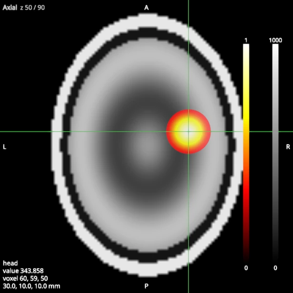
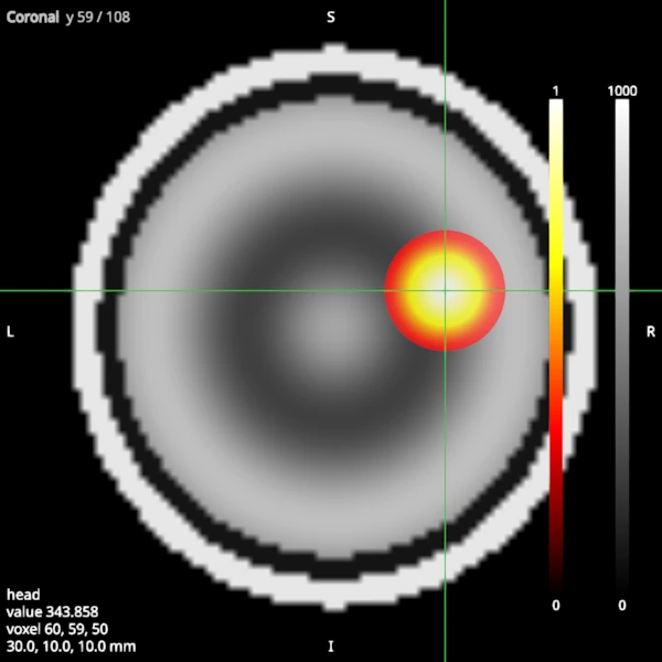
This example builds a synthetic head and a map of a blob inside it, shows the map over the head with a threshold and a colour bar, and saves screenshots of the axial and coronal views. Screenshots are drawn off screen, with no window: the same calls work in a script on a server with no display.

import numpy as np

from larmor.types import Volume
from larmor.viewer import Category, Colormap, OptionName, Viewer, ViewKind

A synthetic head

A 2 mm image of an ellipsoid with a bright scalp, dark fluid under it, and a brain whose intensity rises and falls with the distance from its centre, like grey and white matter. The affine puts the image’s centre at the world origin (world coordinates are in mm, RAS+).

shape = (90, 108, 90)
affine = np.diag([2.0, 2.0, 2.0, 1.0])
affine[:3, 3] = -np.array(shape)  # half the extent in mm: the centre at 0
i, j, k = np.indices(shape, dtype=np.float32)
x, y, z = (2 * i / shape[0] - 1, 2 * j / shape[1] - 1, 2 * k / shape[2] - 1)
r = np.sqrt((x / 0.8) ** 2 + (y / 0.9) ** 2 + (z / 0.85) ** 2)
t1 = np.select(
    [r < 0.82, r < 0.9, r < 1.0],
    [500 + 250 * np.cos(9 * r), np.full(shape, 80.0), np.full(shape, 900.0)],
    0.0,
).astype(np.float32)
head = Volume(t1, affine)

A map to overlay: a blob in the right hemisphere, peaking at 1 at x = 30 mm, y = 10 mm, z = 10 mm.

world = np.stack([i, j, k], axis=-1) @ affine[:3, :3].T + affine[:3, 3]
distance = np.linalg.norm(world - [30.0, 10.0, 10.0], axis=-1)
blob = Volume(np.exp(-((distance / 15.0) ** 2)).astype(np.float32), affine)

The viewer and its items

add shows objects already in memory without copying them; load reads files instead, for example viewer.load("t1.nii.gz", Category.VOLUMES). The first volume puts the crosshair at the centre of its grid.

To look at the same items in a window, pass them to view: view(volumes=head, overlays=blob) opens the viewer and returns when it closes.

viewer = Viewer()
t1_item = viewer.add(head, Category.VOLUMES, name="head")
blob_item = viewer.add(blob, Category.OVERLAYS, name="blob")
viewer.move_cursor((30.0, 10.0, 10.0))  # through the blob's peak

Each item starts with its minimum and maximum at its data’s range. The overlay is drawn with the hot colormap, transparent up to 0.3, at 80% opacity, and both items show a colour bar at the right edge of the 2D views.

viewer.set(blob_item.id, OptionName.COLORMAP, Colormap.HOT)
viewer.set(blob_item.id, OptionName.THRESHOLD, 0.3)
viewer.set(blob_item.id, OptionName.OPACITY_2D, 0.8)
viewer.set(Category.VOLUMES, OptionName.MAXIMUM, 1000.0)
viewer.set(Category.VOLUMES, OptionName.COLOUR_BAR, True)
viewer.set(blob_item.id, OptionName.COLOUR_BAR, True)

Screenshots

screenshot draws one view as the window would show it, with the crosshair, the orientation letters, the crosshair’s readout and the colour bars, and writes the image to a file. The size is in the window’s units (logical pixels).

viewer.screenshot(ViewKind.AXIAL, "viewer_overlay_axial.png", size=(600, 600))
viewer.screenshot(ViewKind.CORONAL, "viewer_overlay_coronal.png", size=(600, 600))

The readout at the cursor reports the main volume (the head), in its own units.

readout = viewer.readout()
print(f"{readout.name} at {readout.position} mm: {readout.value:.1f}")
assert readout.voxel == (60, 59, 50)

head at (30.0, 10.0, 10.0) mm: 343.9