A brain in the viewer

This example shows a brain in the viewer: the simulated brain of the ISMRM 2015 Tractography Challenge, with its T1-like image and diffusion-weighted images on a 2 mm grid. larmor.data downloads it once (about 41 MB) into a cache folder and returns the paths of its files; later runs use the cached copy. The example fits DTI to the diffusion images and shows the fractional anisotropy (FA) over the T1-like image, on an axial and a sagittal slice.

The data is simulated, from the challenge’s Zenodo record (https://doi.org/10.5281/zenodo.572345, CC BY 4.0). Please cite: Maier-Hein KH et al. The challenge of mapping the human connectome based on diffusion tractography. Nature Communications 8 (2017) 1349.

# needs: example-data (the tests run it only when LARMOR_DATA_DIR is set)

import numpy as np

from larmor.data import fetch_ismrm2015
from larmor.dwi import DTIModel, create_brain_mask, mean_b0
from larmor.io import load_dwi
from larmor.types import Volume
from larmor.viewer import Category, Colormap, OptionName, Viewer, ViewKind

Downloading the data and fitting DTI

files = fetch_ismrm2015()
dwi, gtab = load_dwi(files["dwi"], files["bvals"], files["bvecs"])
mask = create_brain_mask(mean_b0(dwi, gtab))
fit = DTIModel().fit(dwi, gtab, mask=mask)

FA over the T1-like image

load reads the T1-like image from its file; add shows the FA map already in memory, on its own grid. Below the threshold the FA is transparent, so only the white matter is coloured. The screenshots hide the crosshair and the text, so they show only the data.

viewer = Viewer()
viewer.load(files["t1"], Category.VOLUMES)
fa = viewer.add(Volume(fit.fa, dwi.affine), Category.OVERLAYS, name="FA")
viewer.set(fa.id, OptionName.COLORMAP, Colormap.HOT)
viewer.set(fa.id, OptionName.THRESHOLD, 0.2)
viewer.set(fa.id, OptionName.OPACITY_2D, 0.8)

shape = np.array(dwi.data.shape[:3])
centre = dwi.affine[:3, :3] @ ((shape - 1) / 2) + dwi.affine[:3, 3]
viewer.move_cursor(tuple(centre + [8.0, 0.0, 4.0]))
viewer.toggle_crosshair()
viewer.zoom(ViewKind.SAGITTAL, 1.3)
viewer.screenshot(
    ViewKind.AXIAL, "viewer_real_axial.png", size=(600, 600), overlay=False
)
viewer.screenshot(
    ViewKind.SAGITTAL, "viewer_real_sagittal.png", size=(900, 600), overlay=False
)
print(f"{int((fit.fa > 0.2).sum())} voxels have an FA above the threshold")

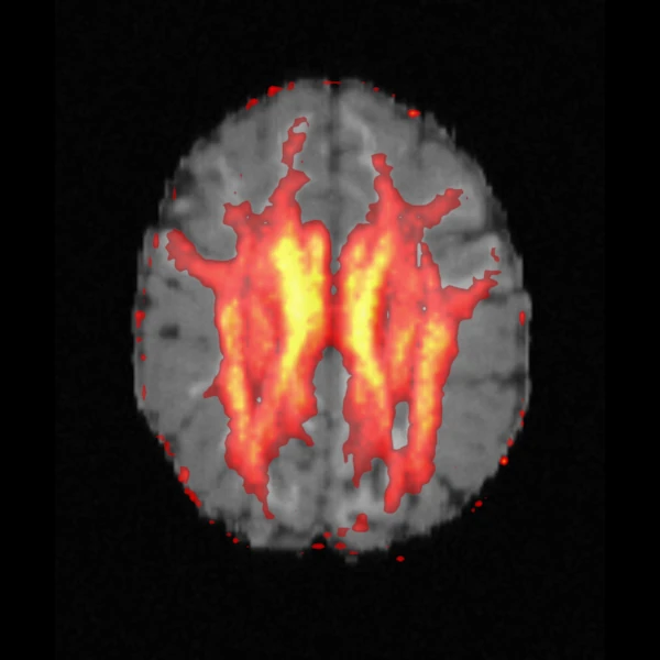
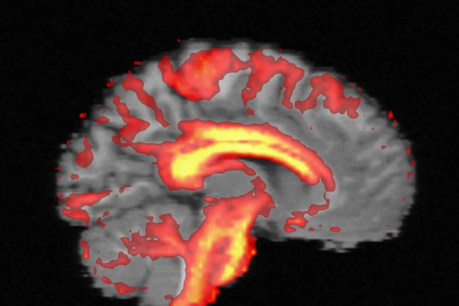
Data: ISMRM 2015 Tractography Challenge (Maier-Hein et al., Nat Commun 8 (2017) 1349), CC BY 4.0.

56096 voxels have an FA above the threshold