Fitting FODs to a synthetic signal

Spherical deconvolution estimates a fibre orientation distribution (FOD) in each voxel: how much of the voxel’s fibres runs in each direction. It models the signal as the sum of the signals of single fibres, each the white matter response turned to point along the fibre, and finds the distribution of fibres that gives back the measured signal.

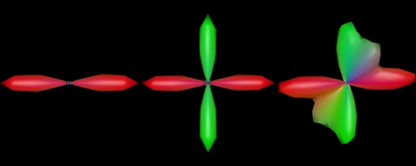
This example simulates the signal of three voxels, with one fibre, two crossing at right angles and three crossing, at one b-value with 64 directions; fits their FODs with a known response; prints how many fibres each FOD shows and how far its peaks lie from the true fibres; and draws the FODs as glyphs.

SDModel uses generalized Richardson-Lucy (GRL; Guo et al. 2020) by default, whose FOD solver is damped Richardson-Lucy (Dell’Acqua et al. 2010), reimplemented from MRIToolkit. Guo F, Leemans A, Viergever MA, Dell’Acqua F, De Luca A. NeuroImage 218 (2020) 116948. Dell’Acqua F, Scifo P, Rizzo G, et al. NeuroImage 49 (2010) 1446-1458.

import numpy as np

from larmor.sd import SDModel, build_response_functions, find_peaks
from larmor.types import GradientTable, Volume
from larmor.viewer import Category, Viewer, ViewKind

The acquisition

One b=0 image and 64 directions at b=2500 s/mm^2, spread evenly over the sphere.

n = 64
z = 1 - (2 * np.arange(n) + 1) / n
azimuth = np.pi * (3 - np.sqrt(5)) * np.arange(n)
radius = np.sqrt(1 - z**2)
directions = np.stack([radius * np.cos(azimuth), radius * np.sin(azimuth), z], axis=1)
gtab = GradientTable(
    np.concatenate([[0.0], np.full(n, 2500.0)]),
    np.vstack([np.zeros(3), directions]),
)

The signal

A single fibre is a tensor with a diffusivity of 1.7e-3 mm^2/s along it and 0.3e-3 across it. Each voxel’s signal is the mean of its fibres’ signals, with a little noise (signal-to-noise ratio 50 at b=0).

AXIAL, RADIAL = 1.7e-3, 0.3e-3


def fibre_signal(fibre: np.ndarray) -> np.ndarray:
    """The signal of one fibre along a unit vector, 1 at b=0."""
    cosines = gtab.bvecs @ fibre
    signal: np.ndarray = np.exp(-gtab.bvals * (RADIAL + (AXIAL - RADIAL) * cosines**2))
    return signal


x, y = np.array([1.0, 0.0, 0.0]), np.array([0.0, 1.0, 0.0])
oblique = np.array([1.0, 1.0, 1.0]) / np.sqrt(3)
fibres = [[x], [x, y], [x, y, oblique]]
rng = np.random.default_rng(0)
data = np.zeros((3, 1, 1, n + 1), np.float32)
for i, voxel in enumerate(fibres):
    signal = np.mean([fibre_signal(f) for f in voxel], axis=0)
    data[i, 0, 0] = 1000 * signal + rng.normal(0, 20, n + 1)
dwi = Volume(data, np.diag([2.0, 2.0, 2.0, 1.0]))

The fit

The white matter response is given here, as the tensor of a single fibre; on real data build_response_functions estimates it from the voxels of highest FA. The FODs come back as SH coefficients up to degree 8, in world coordinates.

mask = np.ones((3, 1, 1), bool)
responses = build_response_functions(
    dwi, gtab, mask, wm_eigen_vals=[AXIAL, RADIAL, RADIAL]
)
fit = SDModel(responses, lmax=8).fit(dwi, gtab, mask=mask)
fod = fit.fods[0]

peaks = find_peaks(fod, num_peaks=3, relative_threshold=0.25)
for i, voxel in enumerate(fibres):
    found = peaks.directions[i, 0, 0][np.isfinite(peaks.amplitudes[i, 0, 0])]
    errors = [np.degrees(np.arccos(np.max(np.abs(found @ f)))) for f in voxel]
    print(
        f"{len(voxel)} fibre(s): {len(found)} peak(s), "
        f"largest error {max(errors):.1f} degrees"
    )

1 fibre(s): 1 peak(s), largest error 0.5 degrees
2 fibre(s): 2 peak(s), largest error 0.9 degrees
3 fibre(s): 3 peak(s), largest error 9.9 degrees

The FODs as glyphs

Each glyph is the FOD’s amplitude in every direction, coloured by direction: red left to right, green front to back, blue up and down. The screenshot hides the crosshair and the text, so it shows only the data.

viewer = Viewer()
viewer.add(Volume(fod.astype(np.float32), dwi.affine), Category.FODS, name="FOD")
viewer.toggle_crosshair()
viewer.screenshot(
    ViewKind.AXIAL, "fod_fit_synthetic.png", size=(600, 240), overlay=False
)