FODs, peaks and asymmetric FODs of a simulated brain

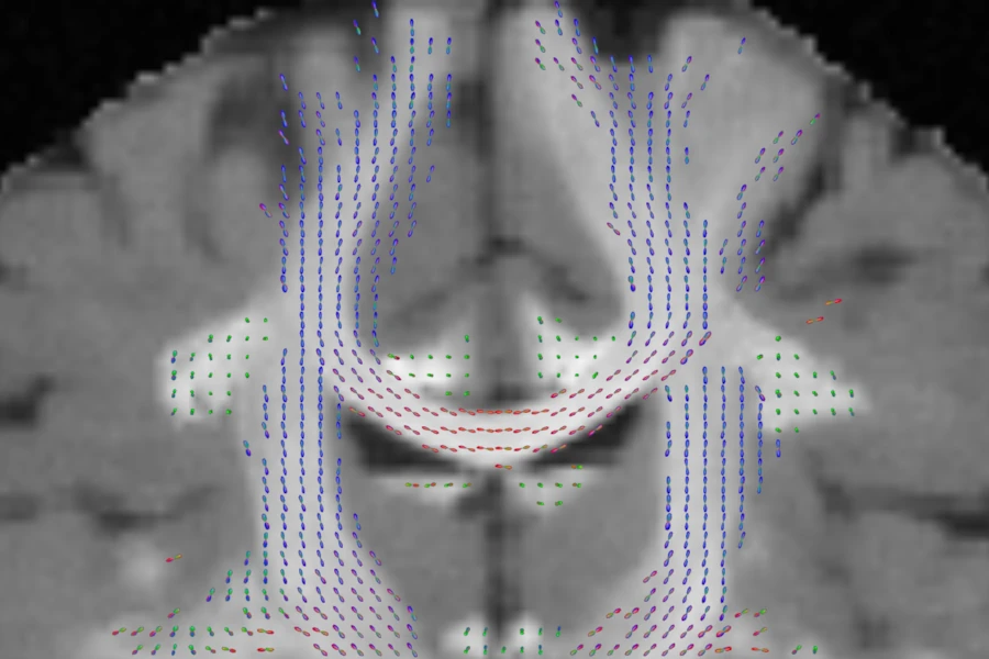
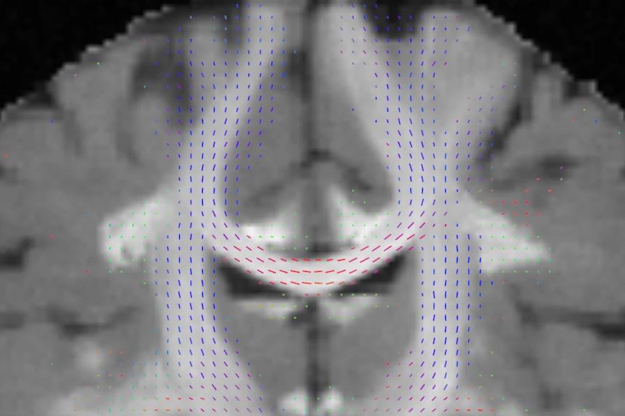
This example estimates fibre orientation distributions (FODs) by spherical deconvolution in the simulated brain of the ISMRM 2015 Tractography Challenge, finds their peaks, and, as an ad hoc illustration, makes asymmetric FODs by averaging each voxel’s neighbours. It shows each over the T1-like image on a coronal slice, where the corpus callosum arches from left to right above the ventricles and the corticospinal tracts run up and down beside it.

The data is simulated: diffusion-weighted images at 2 mm with 32 directions at b=1000 s/mm^2, and a T1-like image, from the challenge’s Zenodo record (https://doi.org/10.5281/zenodo.572345, CC BY 4.0). Please cite: Maier-Hein KH et al. The challenge of mapping the human connectome based on diffusion tractography. Nature Communications 8 (2017) 1349.

The FODs are fitted with GRL (Guo et al., NeuroImage 218 (2020) 116948) and its damped Richardson-Lucy solver (Dell’Acqua et al., NeuroImage 49 (2010) 1446-1458), reimplemented from MRIToolkit; the peaks are found as by sh2peaks of MRtrix3 (Tournier et al., NeuroImage 202 (2019) 116137).

# needs: example-data (the tests run it only when LARMOR_DATA_DIR is set)

import numpy as np

from larmor.data import fetch_ismrm2015
from larmor.dwi import create_brain_mask, mean_b0
from larmor.io import load_dwi
from larmor.sd import SDModel, build_response_functions, find_peaks, fit_sh
from larmor.viewer import Category, OptionName, Viewer, ViewKind

The data and the FOD fit

fetch_ismrm2015 downloads the data once (about 41 MB) and returns the paths of its files. The white matter response is estimated from the data, and the FODs are fitted up to degree 6, the most that 32 directions support.

files = fetch_ismrm2015()
dwi, gtab = load_dwi(files["dwi"], files["bvals"], files["bvecs"])
mask = create_brain_mask(mean_b0(dwi, gtab))
responses = build_response_functions(dwi, gtab, mask)
fit = SDModel(responses, lmax=6).fit(dwi, gtab, mask=mask)
fod = dwi.with_data(fit.fods[0].astype(np.float32))

FOD glyphs

The cursor sets the slices: here a coronal slice 20 mm above the centre of the image. The screenshots hide the crosshair and the text, so they show only the data. A minimum anisotropy hides the round FODs of grey matter and CSF, and a threshold of a fifth of the image’s largest amplitude hides the small ones.

shape = np.array(dwi.data.shape[:3])
centre = dwi.affine[:3, :3] @ ((shape - 1) / 2) + dwi.affine[:3, 3]
focus = tuple(centre + [0.0, 0.0, 20.0])

viewer = Viewer()
viewer.load(files["t1"], Category.VOLUMES)
glyphs = viewer.add(fod, Category.FODS, name="FOD")
viewer.set(glyphs.id, OptionName.ANISOTROPY, 0.3)
viewer.set(glyphs.id, OptionName.THRESHOLD, 0.2)
viewer.move_cursor(focus)
viewer.toggle_crosshair()
viewer.zoom(ViewKind.CORONAL, 2.5, about=focus)
viewer.screenshot(
    ViewKind.CORONAL, "fods_ismrm_glyphs.png", size=(900, 600), overlay=False
)

Data: ISMRM 2015 Tractography Challenge (Maier-Hein et al., Nat Commun 8 (2017) 1349), CC BY 4.0.

Peaks

find_peaks finds the maxima of each FOD, up to 3 here, largest first. A peaks image holds the direction of each peak scaled by its amplitude, 3 values per peak, NaN where a voxel has fewer peaks; the viewer draws each as a short line.

peaks = find_peaks(fod.data.astype(np.float64), mask=mask, num_peaks=3)
vectors = peaks.directions * peaks.amplitudes[..., None]
# The small peaks of grey matter and CSF are left out.
largest = np.nanpercentile(peaks.amplitudes[..., 0][mask], 99)
vectors[~(peaks.amplitudes >= 0.2 * largest)] = np.nan
peaks_image = dwi.with_data(vectors.reshape(*vectors.shape[:3], 9).astype(np.float32))
n_found = np.isfinite(peaks.amplitudes).sum(axis=-1)
print(f"{np.mean(n_found[mask] >= 2):.0%} of the brain's voxels have two peaks or more")

viewer.set(glyphs.id, OptionName.VISIBLE, False)
viewer.add(peaks_image, Category.PEAKS, name="peaks")
viewer.screenshot(
    ViewKind.CORONAL, "fods_ismrm_peaks.png", size=(900, 600), overlay=False
)

39% of the brain's voxels have two peaks or more

Asymmetric FODs

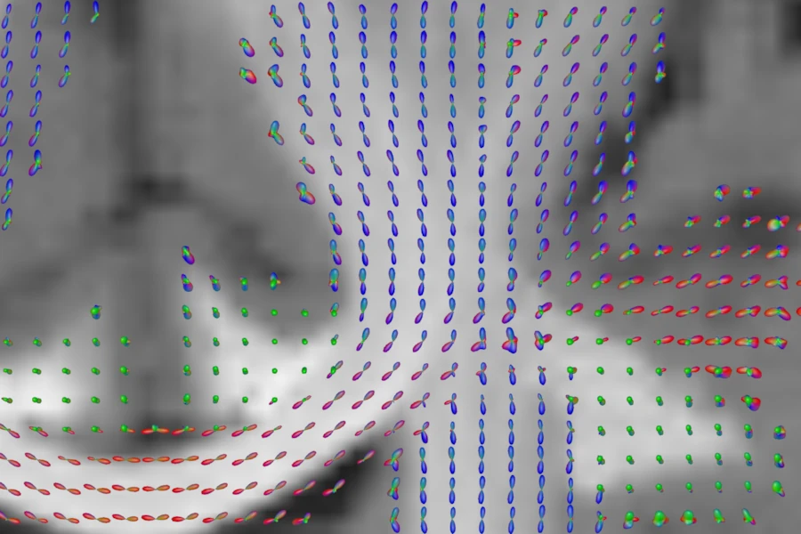
Larmor reads and draws asymmetric FODs, which may differ between the two ends of a direction, but does not estimate them. The asymmetric FODs here are an ad hoc illustration made for this picture, not a method of Larmor nor a published filter. They are made from the symmetric FODs: in each direction, a voxel takes the FODs of its 26 neighbours that lie that way, weighted by how closely they do (the cosine of the angle, to the fourth power). Where a bundle bends or ends, the two ends of a lobe then differ. It is done on the few coronal slices around the one shown, with the FODs as amplitudes on 300 directions.

fit_sh turns amplitudes into SH coefficients; the matrix that does the opposite, from coefficients to amplitudes on these directions, is the inverse of the fit of each direction alone.

n = 300
z = 1 - (2 * np.arange(n) + 1) / n
azimuth = np.pi * (3 - np.sqrt(5)) * np.arange(n)
radius = np.sqrt(1 - z**2)
dirs = np.stack([radius * np.cos(azimuth), radius * np.sin(azimuth), z], axis=1)
to_amplitudes = np.linalg.pinv(fit_sh(np.eye(n), dirs, 6))

j = int(round(np.linalg.solve(dwi.affine[:3, :3], focus - dwi.affine[:3, 3])[1]))
slab = fod.data[:, j - 2 : j + 3].astype(np.float64) @ to_amplitudes
filtered = np.zeros_like(slab[:, 1:4])
weights = np.zeros(n)
for offset in np.ndindex(3, 3, 3):
    step = np.array(offset) - 1
    if not step.any():
        continue
    towards = dwi.affine[:3, :3] @ step
    weight = np.clip(dirs @ (towards / np.linalg.norm(towards)), 0, None) ** 4
    shifted = np.roll(slab, tuple(-step), axis=(0, 1, 2))[:, 1:4]
    filtered += weight * shifted
    weights += weight
filtered /= weights
asymmetric = np.zeros((*fod.data.shape[:3], 49), np.float32)
asymmetric[:, j - 1 : j + 2] = fit_sh(filtered, dirs, 6, full=True)
asymmetric[~mask] = 0

# The view zooms in on the right hemisphere, where fibres of the corpus callosum
# turn upwards and end.

viewer.set(Category.PEAKS, OptionName.VISIBLE, False)
lobes = viewer.add(dwi.with_data(asymmetric), Category.FODS, name="asymmetric")
viewer.set(lobes.id, OptionName.ANISOTROPY, 0.3)
bend = tuple(np.array(focus) + [35.0, 0.0, 0.0])
viewer.zoom(ViewKind.CORONAL, 2.0, about=bend)
viewer.screenshot(
    ViewKind.CORONAL, "fods_ismrm_asymmetric.png", size=(900, 600), overlay=False
)