Tractograms in the viewer

A tractogram is drawn as lines in the 2D views and the 3D view. Its options set how its streamlines are coloured (by direction, in one colour, or one colour per tractogram), what share of them is drawn, how many points each one keeps, and, in the 2D views, the slab: only the parts of streamlines within a few millimetres of the slice are drawn, so a slice shows what passes through it.

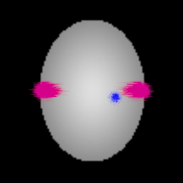
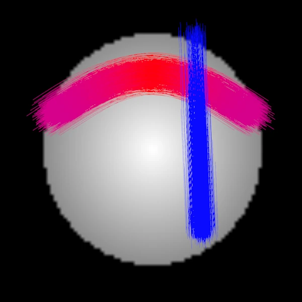
This example builds a synthetic head and two bundles of streamlines, one running left to right and one running up and down, and saves screenshots of the axial and coronal views with the slab, and of the 3D view with a subset of the streamlines.

import numpy as np

from larmor.types import Tractogram, Volume
from larmor.viewer import (
    CameraPreset,
    Category,
    Colouring,
    OptionName,
    Viewer,
    ViewKind,
)

A synthetic head

A 2 mm image of an ellipsoid, centred at the world origin (world coordinates are in mm, RAS+).

shape = (90, 108, 90)
affine = np.diag([2.0, 2.0, 2.0, 1.0])
affine[:3, 3] = -np.array(shape)  # half the extent in mm: the centre at 0
i, j, k = np.indices(shape, dtype=np.float32)
x, y, z = (2 * i / shape[0] - 1, 2 * j / shape[1] - 1, 2 * k / shape[2] - 1)
r = np.sqrt((x / 0.8) ** 2 + (y / 0.9) ** 2 + (z / 0.85) ** 2)
head = Volume(np.where(r < 0.9, 600 - 300 * r, 0).astype(np.float32), affine)

Two bundles

A Tractogram holds the points of all its streamlines one after the other, and the offsets where each one starts. The first bundle arches from left to right over the middle of the brain, like the corpus callosum; the second runs from the top of the brain down through the right hemisphere, like a corticospinal tract.

rng = np.random.default_rng(0)
n, length = 2000, 60
t = np.linspace(0, 1, length, dtype=np.float32)


def bundle(curve: np.ndarray, spread: float) -> np.ndarray:
    """n copies of a curve, each shifted at random by about spread mm."""
    shifts = rng.normal(scale=spread, size=(n, 1, 3)).astype(np.float32)
    return curve[None] + shifts


arch = np.stack([120 * t - 60, np.zeros_like(t), 20 + 25 * np.sin(np.pi * t)], -1)
column = np.stack([25 + 5 * t, -10 + 5 * t, 70 - 120 * t], -1)
streamlines = np.concatenate([bundle(arch, 4.0), bundle(column, 3.0)])
points = streamlines.reshape(-1, 3)
offsets = np.arange(0, len(points) + 1, length, dtype=np.int64)
tracts = Tractogram(points, offsets)

The viewer and its items

Tractograms are added like volumes; load reads a TCK or TRK file instead. The cursor, which sets the slices, goes through both bundles.

viewer = Viewer()
# The screenshots hide the crosshair and the text, so they show only the data.
viewer.toggle_crosshair()
viewer.toggle_overlay()
viewer.add(head, Category.VOLUMES, name="head")
item = viewer.add(tracts, Category.TRACTOGRAMS, name="bundles")
viewer.move_cursor((25.0, 0.0, 20.0))

The slab

Each streamline starts coloured by its direction: red left to right, green front to back, blue up and down. In the 2D views the slab is on, 5 mm thick by default: the axial view shows where the column crosses the slice, the coronal view shows the arch along it. Here it is 10 mm, to show a little more of each bundle.

viewer.set(item.id, OptionName.SLAB_THICKNESS, 10.0)
viewer.screenshot(ViewKind.AXIAL, "viewer_tracts_axial.png", size=(600, 600))
viewer.screenshot(ViewKind.CORONAL, "viewer_tracts_coronal.png", size=(600, 600))

A subset in one colour

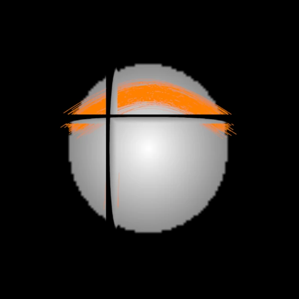
With millions of streamlines, a subset is often enough to see the shape of the tractogram, and much faster to draw. The subset is a percentage of the streamlines, taken at random, the same ones each time. Here a quarter of them, in orange, seen from the front in the 3D view, without the head’s volume rendering (its 3D opacity at 0), which would hide the lines inside it.

viewer.set(item.id, OptionName.SUBSET, 25.0)
viewer.set(item.id, OptionName.COLOURING, Colouring.SINGLE)
viewer.set(item.id, OptionName.COLOUR, "#ff8000")
viewer.set(Category.VOLUMES, OptionName.OPACITY_3D, 0.0)
viewer.set_camera(ViewKind.THREE_D, CameraPreset.CORONAL)
viewer.screenshot(ViewKind.THREE_D, "viewer_tracts_3d.png", size=(600, 600))
print(f"{tracts.num_streamlines} streamlines, {len(points)} points")

4000 streamlines, 240000 points