Tract profiles: FA along a bundle#

A tract profile describes a bundle by the values of a map, such as FA, at points along its length, so that subjects or groups can be compared point by point rather than by one mean over the whole bundle. Larmor orients the streamlines so that all run the same way, resamples each to the same number of points, samples the map at those points, and averages the streamlines’ values at each point, weighting each streamline by how close it lies to the bundle’s core.

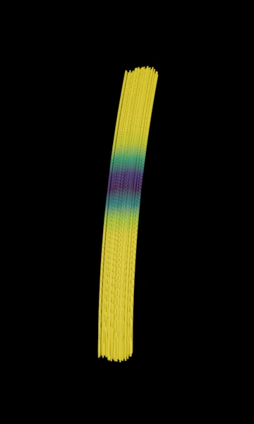
This example builds a synthetic bundle running from the brainstem up to the cortex through an FA map with a lesion halfway, computes its FA profile, prints it, plots it with matplotlib (not a dependency of Larmor: pip install matplotlib), and colours the bundle by the profile in the viewer.

Tract profiles follow Yeatman JD et al. Tract profiles of white matter properties: automating fiber-tract quantification. PLoS One 7 (2012) e49790; and Chandio BQ et al. Bundle analytics, a computational framework for investigating the shapes and profiles of brain pathways across populations. Sci Rep 10 (2020) 17149.

import tempfile
from pathlib import Path

import numpy as np
from matplotlib.figure import Figure

from larmor.io import write_tsf
from larmor.tractography import tract_profile
from larmor.types import Tractogram, Volume
from larmor.viewer import (
    CameraPreset,
    Category,
    Colormap,
    OptionName,
    TractStyle,
    Viewer,
    ViewKind,
)

An FA map with a lesion#

A 2 mm image centred at the world origin, with FA 0.7 everywhere except a lesion of lower FA centred at z = 10 mm.

shape = (60, 60, 60)
affine = np.diag([2.0, 2.0, 2.0, 1.0])
affine[:3, 3] = -np.array(shape)  # half the extent in mm: the centre at 0
i, j, k = np.indices(shape, dtype=np.float32)
z = 2 * k - 60
fa = Volume(0.7 - 0.3 * np.exp(-(((z - 10) / 8) ** 2)), affine)

A bundle like a corticospinal tract#

500 streamlines from z = -50 mm (the brainstem end) up to z = 50 mm, bending outwards towards the top. Tracking stores streamlines in either direction, so half of them run from the top down.

rng = np.random.default_rng(0)
lines = []
for s in range(500):
    n = int(rng.integers(40, 80))
    t = np.linspace(0.0, 1.0, n)
    shift = rng.normal(scale=2.0, size=2)
    line = np.stack(
        [
            -15 + shift[0] - 10 * t**2,
            shift[1] + np.zeros(n),
            -50 + 100 * t,
        ],
        axis=1,
    )
    lines.append(line[::-1] if s % 2 else line)
offsets = np.concatenate([[0], np.cumsum([len(line) for line in lines])])
bundle = Tractogram(np.concatenate(lines), offsets)

The profile#

20 points along the bundle. Without a start point, the profile starts at the end that is left, posterior or inferior along the bundle’s main axis: here the inferior one, the brainstem. profile.reversed says which streamlines were reversed to run that way. Real data comes from files: load_tractogram, load_volume, or lar tract-profile bundle.tck fa.nii.gz profile.csv.

profile = tract_profile(bundle, {"fa": fa}, num_points=20)
print(f"{profile.reversed.sum()} of {bundle.num_streamlines} streamlines reversed")
print(" point   z (mm)   FA")
for n, (core, value) in enumerate(zip(profile.core, profile.values["fa"], strict=True)):
    bar = "#" * round(60 * value)
    print(f"{n:6d} {core[2]:8.1f} {value:6.3f} {bar}")

of 500 streamlines reversed
 point   z (mm)   FA
  -50.0  0.700 ##########################################
  -44.7  0.700 ##########################################
  -39.4  0.700 ##########################################
  -34.1  0.700 ##########################################
  -28.8  0.700 ##########################################
  -23.5  0.700 ##########################################
  -18.2  0.700 ##########################################
  -12.9  0.700 ##########################################
   -7.7  0.698 ##########################################
   -2.4  0.672 ########################################
    2.9  0.563 ##################################
    8.1  0.417 #########################
   13.4  0.452 ###########################
   18.7  0.605 ####################################
   23.9  0.685 #########################################
   29.1  0.699 ##########################################
   34.4  0.700 ##########################################
   39.6  0.700 ##########################################
   44.8  0.700 ##########################################
   50.0  0.700 ##########################################

The profile as a plot#

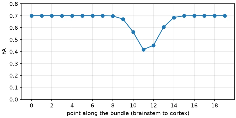
The lesion shows as the dip in the middle of the profile. profile.write_csv saves the table, one row per point; here it is drawn with matplotlib.

figure = Figure(figsize=(6, 3), layout="constrained")
axes = figure.add_subplot()
axes.plot(np.arange(len(profile.core)), profile.values["fa"], marker="o")
axes.set_xlabel("point along the bundle (brainstem to cortex)")
axes.set_ylabel("FA")
axes.set_ylim(0, 0.8)
axes.set_xticks(range(0, len(profile.core), 2))
axes.grid(alpha=0.3)
figure.savefig("tract_profile_plot.png", dpi=150)

The bundle coloured by its profile#

profile.segments(bundle) gives each point of the bundle the index of its profile point; indexing the profile with it gives each point its segment’s FA. Written as a TSF file, these values colour the bundle in the viewer, through a colormap from the lowest FA to the highest (lar tract-profile --tsf-prefix writes the same files). The screenshot shows the bundle alone, as tubes.

folder = Path(tempfile.mkdtemp())
per_point = profile.values["fa"][profile.segments(bundle)].astype(np.float32)
write_tsf(per_point, bundle.offsets, folder / "bundle_fa.tsf")

viewer = Viewer()
item = viewer.add(bundle, Category.TRACTOGRAMS, name="bundle")
viewer.set(item.id, OptionName.VALUES_FILE, str(folder / "bundle_fa.tsf"))
viewer.set(item.id, OptionName.COLORMAP, Colormap.VIRIDIS)
viewer.set(item.id, OptionName.MINIMUM, float(per_point.min()))
viewer.set(item.id, OptionName.MAXIMUM, float(per_point.max()))
viewer.set(item.id, OptionName.STYLE, TractStyle.TUBES)
viewer.set_camera(ViewKind.THREE_D, CameraPreset.CORONAL)
viewer.rotate_camera(20.0, 0.0)
viewer.zoom(ViewKind.THREE_D, 0.85)
viewer.screenshot(
    ViewKind.THREE_D, "tract_profile_3d.png", size=(360, 600), overlay=False
)